Code as a Liberal Art, Spring 2024
Unit 1, Lesson 4 — Thursday, February 15
Table of contents
Topics today: (Click each to jump down to the corresponding section.)
- Images and pixels
- Algorithms and images: filtering
- Algorithms and images: generation
- Algorithms and Images: combination
- Wrapping up & homework
I. Images and pixels
Let's think about how we can access, manipulate, generate, and save files from within Python by focusing on image files. Exploring how we work with images in Python will link to several of "principles" of digital media that we considered when reviewing the Manovich reading, like numerical representation and modularity.
Digital images are comprised of pixels, essentially the atomic unit of digital imagery.
There are many different types of digital image files, usually called formats. You already know many of these: JPEG, PNG, TIFF, GIF, bitmaps, etc. Each of these different formats uses different techniques and algorithms for encoding a visual image as digital data.
a. Image formats (and transcoding)
The Python Image Library (PIL) makes it very easy to convert between different image formats. Incidentally, this offers us a really nice demonstration of the principle that Manovich called "transcoding: a process of translating a digital object from one encoding scheme into another. For example, converting one type of image file into a different type.
When you save a file using PIL, the save() command
examines the name of the file that you specify, and tries to
determine what type of encoding is implied by that, and
automatically converts the image to this encoding before
saving. Quite convenient. (Refer back
to Lesson 1, part IV for
some background & explanation on file types
and extensions.)
Let's briefly consider this short program:
import sys
from PIL import Image

if len(sys.argv) != 2:
    exit("This command requires one argument: the name of an image file")

img = Image.open( sys.argv[1] )

img.save( sys.argv[1] + ".jpg" )
img.save( sys.argv[1] + ".gif" )
img.save( sys.argv[1] + ".tiff" )
img.save( sys.argv[1] + ".png" )
If you run that command and specify an image filename, you shuold see four new image files in the same folder in which you ran it:
fire.jpg.gif
fire.jpg.jpg
fire.jpg.png
fire.jpg.tiff
And you should be able to open each of these, seeing the same content. Given that each of these image formats uses different internal data structures and encoding algorithms, you may actually be able to disceren some subtle differences in details of the image.
(Note that the "double" extension shouldn't be an issue. Your operating system will pay attention only to the last few characters to determine the file type.)
This transcoding file converter tool might not seem that useful, since you could easily do the same thing in Preview (on Mac) or the equivalent tool on Windows. But maybe you might see some potential usefulness here if you needed to batch convert many files from one format to another.
b. Pixels as a grid
Regardless of what image format you are working with, you can think of images as comprising pixels, each one a small dot of color, arranged in a grid, each dot of color encoded as a numerical value.
Sidenote: Are all images really grids of pixels? Strictly speaking, the internal data of many different image file formats is not stored as grids of pixels because many image formats use compression algorithms: efficiency tricks that allow an image to be comprised of less data, and hence a smaller file size. JPEGs are a prime example. But even for image formats that use compression, when you are working with JPEGs (or any image files) in computer programs in most programming languages (like Python), they all nearly always get translated into grids of numerical pixel values to be manipulated by computer program code.
When working on computer programs that work with images, you can think of the pixels of an image as arranged in a grid, with rows and columns. (You can also think of the pixels as as existing in one long list, in which all the rows are stored together in order. We'll talk about this below.)
Generally, the first pixel of an image is the dot located visually at the top-left corner of the image. When we're thinking about pixels in a grid, each pixel will be indicated by two indices, two numbers, refered to as coordinates.
In most computer graphics contexts, the top-left corner of the
pixel grid is indicated with 0,0. The horizontal dimension is
always specified first and is referred to as x, and
the vertical dimension is always specified second and is
referred to as y.

So, what would be the coordinates of this pixel?
It would be 2,3 — remember, we start counting
from 0,0.
What about the coordinates of this pixel?
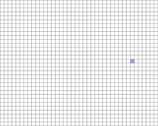
I would not recommend actually trying to count those! Instead
you can approximate. Maybe x=30
and y=15?
Computers require us to be precise, but we can comply with that precision while also being loose and approximate in achieving the goals that we're working toward. We can leave space to play, experiment, estimate, and work by trial-and-error.
We can experiment with this in code with the following short program:
import sys
from PIL import Image

img = Image.open( sys.argv[1] )

one_pixel = img.getpixel( (0,0) )
print(one_pixel)

img.putpixel( (10,10), (255,0,0) )

img.save("new.jpg")
This program requires a filename to be specified on the command
line (though it has no error handling!). It tries to
open that file as an image, then uses the PIL
command .getpixel()
to retrieve the pixel value at coordinate (0,0),
which it then prints, then it tries to set a pixel
value using the PIL
command .putpixel(),
setting that pixel to (255,0,0), which is red. Then
it saves the image as a JPEG.
If you run that and examine the output, you might find it very hard to actually see that single red pixel. That is because the JPEG image format uses an encoding that recognizes one single pixel value as something that probably needs to be "smoothed out" in a sense. JPEGs are optimized for photographic images and use compression that works well for that but does not work well for things like a single pixel value. Try saving the image as a PNG and note the difference:
import sys
from PIL import Image

img = Image.open( sys.argv[1] )

one_pixel = img.getpixel( (0,0) )
print(one_pixel)

img.putpixel( (10,10), (255,0,0) )

img.save("new.jpg")
img.save("new.png")
What's up with the double parentheses???
One somewhat idiosyncratic thing about the Python Image Library
is that it expects many arguments to its commands to be
specified as tuples, a type of Python data
structure that we will talk about later. This applies to things
like coordinates and color values. In practical
terms, what it means is that when you are
specifying x,y values to PIL, you will usually have
to specify them in parentheses ( ) even if that
pair of numbers is the only argument to the command. This can
look kind of funny, like in the getpixel() line
above. Similarly, in putpixel(), the color value is
specified as three numbers which also much be specified within
parentheses. I often use some extra spaces to help make this
clearer to read, as I have done above. Make sure you don't
forget to do this! You would get an error if you tried to
specify the x,y values to getpixel()
like this:
img.getpixel(0,0) # Wrong!!
But what are those numbers?? What is (19, 25, 15) and (255,0,0)?
c. The numbers of a pixel
Each pixel is usually represented by 3 numbers, but they can also often be represented by 1 or 4 numbers. When one number, it corresponds to a shade of gray. When three numbers, it corresponds to red, green, and blue, which combine to form all the colors that a system can display. When four numbers, the fourth correponds to opacity, usually referred to as alpha: how see-through is this pixel.
Each component of these pixel values generally goes from 0 to 255.
Sidenote: Why 255? Everyone knows computers represent numerical values internally with binary numbers. Binary counting goes like this:
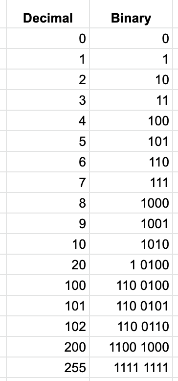
If you scrutinize that, you might start to see some patterns. Two binary digits can represent up to the number 3, three binary digits can represent up to 7. If we continued, you'd see that four binary digits can represent up to 15. The pattern here is that
ndigits in binary can represent2n-1values. (2 to the 2nd power is 4, minus 1 is 3; 2 to the 3rd power is 8, minus 1 is 7; etc.)You may already know that one single binary digit is called a bit (from Binary digIT). You may have also heard the term byte. A byte is defined in digital machinery as eight bits strung together. The name comes from a cutesy play on the term bit. Think of it as a dad joke from a 1950s computer scientist that the world has been stuck with ever since. Sometimes a byte is called a word.
A byte is a common unit of binary data. What is the largest number that can be represented by a byte? Remember
2n-1. Can anyone answer? (Highlight to see.) 255. 2 to the 8th power is 256, minus 1 is 255.So, each pixel is represented by one, three, or four bytes, depending on the type of color, as described above.
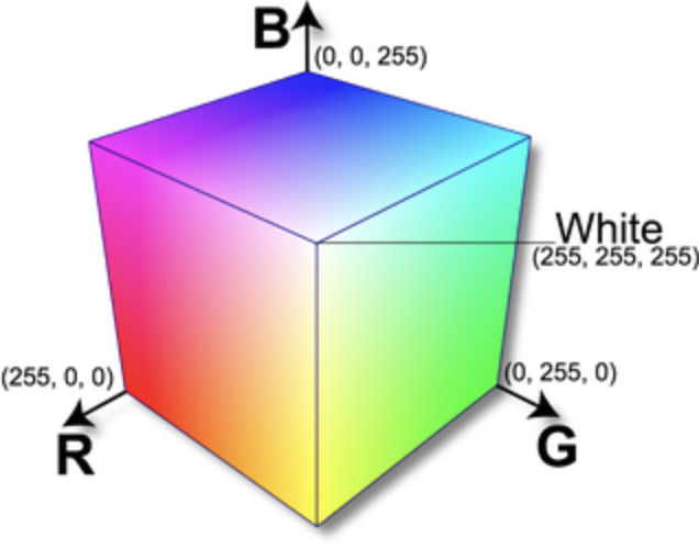
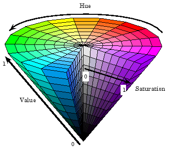
Thinking of color as space. I said that pixels are represented by three color components (red, green, and blue), and that is not always true. There are other models that we think of for representing color. Thinking about these it can be useful to imagine them spatially. In the diagrams below, on the left, we have R, G, B space, as a cube. Pay attention to how red, green, and blue are specified, and how they combine. On the right side is an alternative model called Hue, Saturation, Value. In this scheme, hue is represented by a value 0-360 corresponding to moving around the circular part of this cone; value moves up corresponding to how light or dark the color is; and saturation corresponds to the distance from the center to the edge of the circle. A color with low saturation appears more gray, brightness determines whether that gray would be more white or black, and hue is the actual shade of the color.
I share this with you because when working with color in computer programs, it is often much easier to do more powerful things using the HSV model. Often these different schemes are even called colorspaces, a term you may have encountered in various digital tools like the Adobe Creative Suite. With this representation, we can have one number ranging from 0 to 360 to represent all colors of the spectrum: red, orange, yellow, green, blue, indigo, violet ("ROY G BIV"). With the RGB model, moving through the spectrum like this would be very difficult. We'll see some examples of this in our code for today.
You can work with different color modes in PIL by using
the .convert()
command, which I will illustrate with code in the next section.
II. Algorithms and images: filtering
Let's see how we can apply some algorithmic techniques that we've coded so far to digital images.
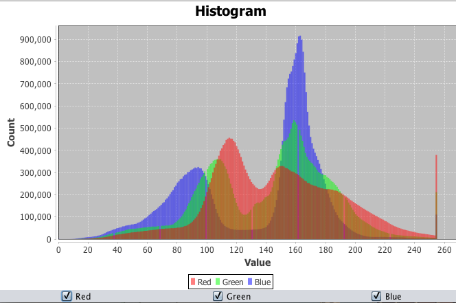
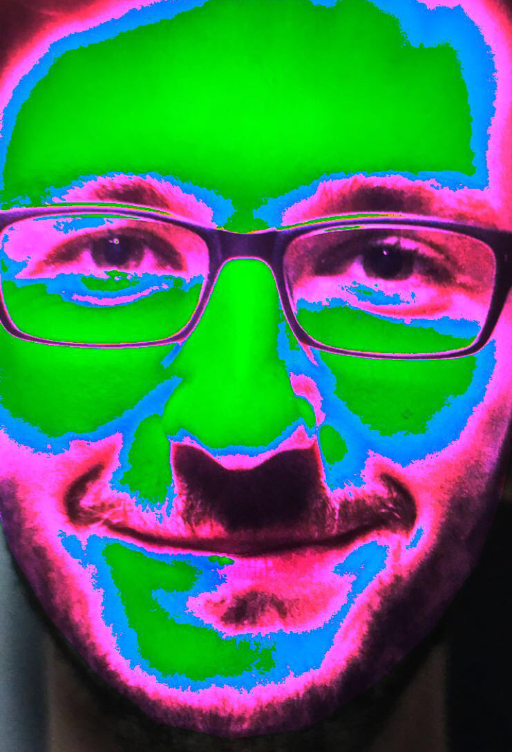
The image on the left is a histogram that shows the relative amounts of various color components (red, green, and blue) in a digital image. The image on the right is the result of a filter applied to replace all colors in the image with only 4 or 5 colors, determined based on the brightness of pixels in the original.
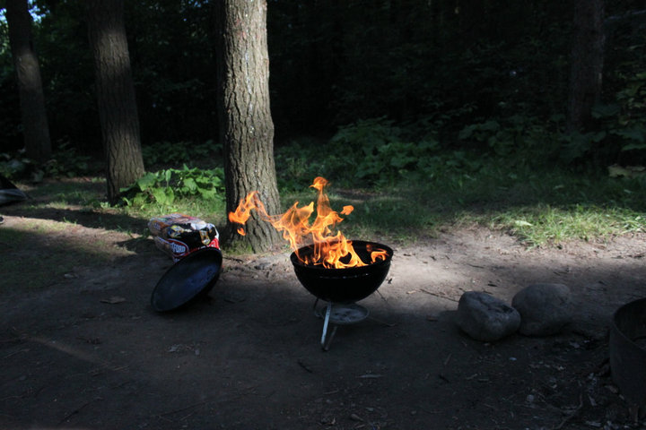
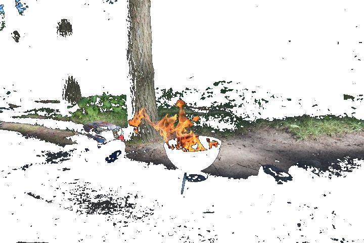
The code sample below opens an image and applies a filtering algorithm which loops over the image, pixel by pixel, checking each one for brightness. Pixels that are below a certain level of brightness are simply replaced with white. A sample output of what this looks like is below.
Example 1 (filter_list.py): Filtering image pixels as a list
import sys
from PIL import Image

img = Image.open( sys.argv[1] )

img_hsv = img.convert(mode="HSV")

img_hsv_data = img_hsv.getdata()

new_img_data = []
for p in img_hsv_data:
    if p[2] < 50:
        new_img_data.append( (0,0,255) )
    else:
        new_img_data.append(p)

img_hsv.putdata(new_img_data)

img_rgb = img_hsv.convert("RGB")
img_rgb.save("filtered.jpg")
Some explanation of that:
img.convert(mode="HSV") converts the input image into
HSV mode so that we can use the HSV scheme described above in
filtering our image.
img_hsv_data = img_hsv.getdata() gets all the
internal pixel data of this image, which is a list, and assigns it
into the variable img_hsv_data. This is a regular
list and we can loop over it and operate on it in the same that we
talked about lists two weeks ago.
new_img_data = [] makes a new empty list, into which
we will put our filtered image data. We are making a copy of the
original image's internal data list into a new data list,
modified in accordance with our filter.
Then we loop over the HSV version of the original image data and
use an if statement to apply our filter. We're
checking p[2] which is the third component of the
pixel value. (Remember that in Python as in most programming
languages, data structures are indexed starting with 0.) In HSV
mode this corresponds to "value", which is the brightness. In this
case we're checking if the brightness is less than 50, a
relatively dark pixel.
If that is true, we're appending (0,0,255) to
our new image data list, which is white in HSV mode. If not
(else) we are simply appending p, which
is the original unfiltered pixel with all its values.
Finally, img_hsv.putdata(new_img_data) puts our new
image data list back into the HSV image.
Then img_rgb = img_hsv.convert("RGB") converts the
image back into RGB mode and assigns that to a new variable, and
the last line saves that new RGB image as a file.
But there is another way we could implement this same filtering algorithm that does not use a list data structure, but rather that loops over the image as a grid of pixels.
Have a look at this code:
Example 2 (filter_grid.py): Filtering image pixels as a grid
import sys
from PIL import Image

img = Image.open( sys.argv[1] )

img_hsv = img.convert(mode="HSV")

(width,height) = img_hsv.size

for x in range(width):
    for y in range(height):
        pixel = img_hsv.getpixel((x,y))
        if pixel[2] < 50:
            img_hsv.putpixel( (x,y), (0,0,255) )

img_rgb = img_hsv.convert(mode="RGB")
img_rgb.save("filtered.jpg")
This does something pretty different which is called
a nested loop, or a loop within a loop. It also
uses the Python range() command which creates a kind
of temporary list of sequential numbers that we can use for
looping.
First we get the size or dimensions of the source
image: (width,height) = img_hsv.size
Then, the outter loop (for x) loops
over the horizontal dimension, from 0
to width. Within that, the
second inner loop (for y) loops over
the vertical dimension, from 0 to height. So for each
horizontal x value, y will loop over
each vertical value.
What will be the actual order that this algorithm visits each pixel?
Highlight to see: (0,0) (0,1) (0,2) ... (1,0) (1,1) (1,2) and so on ... So you might say, in columns
(jump back up to table of contents)III. Algorithms and images: generation
Now let's explore working with algorithms to generate digital images by making numerical patterns. We can do this in the most rudimentary way possible: by manipulating lists of pixels.
As you work with code and computers, you will start to realize that often the most "basic" way of doing something turns out to be the most complicated. The more we try to strip away layers of complexity in computing, the harder tasks become. For example, so-called "high level" programming languages (like Python or Java) are much easier to write than "low level" languages (like C or assembly). All those layers usually add ease of use. They automate the minutia and details of tasks. But working with higher level parts of the system means we often don't get to experience how computers work at more granular levels — it takes you "farther" away from the machine, and from a hands-on grasp of the specific formal properties that we're experimenting with in this unit.
One of the things we're doing in this first unit of the semester as we focus on digital formalism is grapple with some of these lower levels.
Let's start by creating a very small image by building up a list of pixels. Create a new file in VS Code and type the following:
Example 2: Creating a simple 10x10 image
import sys
from PIL import Image

if len(sys.argv) != 2:
    exit("This program requires one argument: the name of the image file that will be created.")

# Make a new 10x10 image
img = Image.new("RGB", (10,10) )

img.save(sys.argv[1])
Try running this. First of all, you'll see that if you don't type one argument you get a helpful error message. But then you should see that whatever filename you pass will be created as a tiny digital image, that is all black. Let's add some color to it by creating pixels:
import sys
from PIL import Image

if len(sys.argv) != 2:
    exit("This program requires one argument: the name of the image file that will be created.")

# Make a new 10x10 image
img = Image.new("RGB", (10,10) )

data = []
for i in range(100):
    pixel = (i, 0, 0)
    data.append( pixel )

img.putdata(data)

img.save(sys.argv[1])
With this code, we're making a new array. Then we are looping
from 0 to 99. That's because a 10x10 image will require 100
pixels, and remember that in computer programs lists almost
always start with 0. Inside that loop, as the
variable i increases from 0 to 99, we're
using i as the red component of a pixel value in
the variable called pixel, then
using append() to add that to a list. Finally, when
the loop is complete, we use a Pillow command
called putdata() to add that list of pixels into
the new image.
Run that and see what it looks like. If you open the resulting image with a program like Preview and zoom in, you should see something like this:
Can you try to do some more interesting things with these pixels values? Here's an attempt:
import sys
from PIL import Image

if len(sys.argv) != 2:
    exit("This program requires one argument: the name of the image file that will be created.")

# Make a new 10x10 image
img = Image.new("RGB", (10,10) )

data = []
for i in range(100):
    pixel = (i, 0, 255-i)
    data.append( pixel )

img.putdata(data)

img.save(sys.argv[1])
What other patterns can you create with that loop?
As a next step, try simply making a larger image. Here I'll make a 400x400 pixel image. That means 160,000 pixels total:
import sys
from PIL import Image

if len(sys.argv) != 2:
    exit("This program requires one argument: the name of the image file that will be created.")

# Make a new 400x400 image
img = Image.new("RGB", (400,400) )

data = []
for i in range(160000):
    pixel = (i, 0, 255-i)
    data.append( pixel )

img.putdata(data)

img.save(sys.argv[1])
This works in some sense. If you open the resulting image and zoom in you'll see a thin stripe of gradient in the top row of the image. But technically this has some errors. The pixel values are going to get very large as the loop increases, larger than 255. So this might create some glitchy images, depending on the image format.
The modulo operator (%). One way
you could improve on this behavior is to use our old friend
the modulo operator: %.
As I've mentioned, modulo is a very powerful idea in computer science and computer programming. If you ever have a variable that you are incrementing, but you want to constrain it to not exceed some maximum value, you can use modulo. In this case, we have a variable that is looping over every pixel in the image, but we want our pixels to stay in the 0-255 range.
Have a look at another example and step through to make sure you understand what's going on here:
>>> for i in range(10):
...   print(i % 3)
...
0
1
2
0
1
2
0
1
2
0
When i is 0, 1, or 2, the remainder
when i is divided by 3 is simply 0, 1, and 2,
respectively. (e.g. 3 goes in to 2 zero times, with a remainder
of 2.) But when i equals 3, the remainder is 0
— because 3 goes in one time, with no remainder. And
when i equals 4, 3 goes in one time with remainder
1. And the pattern continues.
We can use this in our pixel example by incrementing a looping
variable, and applying a % 255 to ensure that the
variable never increases beyond 255:
Example 2: Introducing the modulo operator
import sys
from PIL import Image

if len(sys.argv) != 2:
    exit("This program requires one argument: the name of the image file that will be created.")

# Make a new 400x400 image
img = Image.new("RGB", (400,400) )

data = []
for i in range(160000):
    pixel = (i%255, 0, 0)
    data.append( pixel )

img.putdata(data)

img.save(sys.argv[1])
If you run this, you should see a 400x400 image comprised of small gradients as the red component of the pixel values increase to 255 and then reset to 0.
Play with this new technique and see what you can get. What if you use different modulo values on the red, green, and blue components.
Pixels on the x,y grid. Remember, we can work with pixels on the x,y grid, horizontally and vertically as well. Not just one single list of pixels.
Create a new file in VS Code and type the following:
Example 3: Working with pixels on as a grid
import sys
from PIL import Image

if len(sys.argv) != 2:
    exit("This program requires one argument: the name of the image file that will be created.")

# Make a new 400x400 image
img = Image.new("RGB", (400,400) )

for y in range(400):

    for x in range(400):

        pixel = (x % 255, 0, y % 255)
        img.putpixel( (x,y), pixel )

img.save(sys.argv[1])
This code, called a nested loop, first loops
from 0 to 400 incrementing y each time, and each
time it increments y, it then loops again from 0 to
400, incrementing x each time. That means the code
inside the inner loop will operate on all pixels
one at a time, based on their x,y values. Here I'm
using x to control the red value,
and y to control the blue. Run this and see what
that pattenr looks like.
x,
from left to right, and blue increases with y, from
top to bottom.
Modulo is also very useful to determine even and odd
numbers. If n % 2 is zero, that
means n is divisible by 2, which means that it is
even. Similary if n % 3 is zero, that means it is
divisible by 3, and so on. We can use this fact to create
interesting repetitions and striping behavior:
Example 4: Using modulo and the pixel grid to make stripes
import sys
from PIL import Image

if len(sys.argv) != 2:
    exit("This program requires one argument: the name of the image file that will be created.")

# Make a new 400x400 image
img = Image.new("RGB", (400,400) )

for y in range(400):

    for x in range(400):

        r = 0
        b = 0
        if x % 50 == 0:
            b = 255

        if y % 20 == 0:
            r = 255

        if y % 30 == 0:
            r = 255
            b = 255

        pixel = (r, 0, b)
        img.putpixel( (x,y), pixel )

img.save(sys.argv[1])
As a last step here, we can use the modulo
operator not just checking equality (==)
but checking ranges, with <
and >. Have a look at this example and its
output:
Example 5: Using modulo, the pixel grid, and greater than / less than operators
import sys
from PIL import Image

if len(sys.argv) != 2:
    exit("This program requires one argument: the name of the image file that will be created.")

# Make a new 400x400 image
img = Image.new("RGB", (400,400) )

for y in range(400):

    for x in range(400):

        r = 0
        g = 0
        b = 0
        if x % 50 > 25:
            r = 255

        if y % 50 > 25:
            b = 255

        if x % 100 > 50 and y % 100 > 50:
            g = 255

        pixel = (r, g, b)
        img.putpixel( (x,y), pixel )

img.save(sys.argv[1])
IV. Algorithms and Images: combination
This is as far as we got in class. I encourage you to play with the below examples while doing the homework for this week, and we'll pick up here next week in class.
Example 6: Combining images
import sys
from PIL import Image

if len(sys.argv) != 3:
    exit("This program requires two arguments: the name of two image files to combine.")


# open both images
img1 = Image.open( sys.argv[1] )
img2 = Image.open( sys.argv[2] )

# resize both images so they are no bigger than 400x400
# but preserve the original aspect ratio
img1.thumbnail( (400,400) )
img2.thumbnail( (400,400) )

# make a new image 600x600, with a white background
new_image = Image.new( "RGB", (600,600), "white" )

# paste in the first image to the upper-left corner (0,0)
new_image.paste(img1, (0,0) )

# paste in the second image, to (200,200)
new_image.paste(img2, (200,200) )

# save the resulting image
new_image.save("new.jpg")
Example 7: Combining images with transparency
import sys
from PIL import Image

if len(sys.argv) != 3:
    exit("This program requires two arguments: the name of two image files to combine.")


# open both images
img1 = Image.open( sys.argv[1] )
img2 = Image.open( sys.argv[2] )

# resize both images so they are no bigger than 400x400
# but preserve the original aspect ratio
img1.thumbnail( (400,400) )
img2.thumbnail( (400,400) )

# make a new image 600x600, with a white background
# Note that this image now has an "alpha" component
new_image = Image.new( "RGBA", (600,600), "white" )

# paste in the first image to the upper-left corner (0,0)
new_image.paste(img1, (0,0) )

# add some transparency (alpha) to the second image
img2.putalpha(128)

# paste in the second image, preserving its new transparency
new_image.alpha_composite(img2, (200,200) )

# save the resulting image
# Note that we must convert it to RGB with no alpha to save it as a JPEG
new_image.convert("RGB").save("new.jpg")

# Alternatively, we could have avoided converting by saving it to a
# PNG like this (since PNGs allow alpha):
# new_image.save("new.png")
Example 8: Combining images with transparency based on pixel values of the source image
import sys
from PIL import Image

if len(sys.argv) != 3:
    exit("This program requires two arguments: the name of two image files to combine.")


# open both images
img1 = Image.open( sys.argv[1] )
img2 = Image.open( sys.argv[2] )

# resize both images so they are no bigger than 400x400
# but preserve the original aspect ratio
img1.thumbnail( (400,400) )
img2.thumbnail( (400,400) )

# make a new image 600x600, with a white background
# Note that this image now has an "alpha" component
new_image = Image.new( "RGBA", (600,600), "white" )

# paste in the first image to the upper-left corner (0,0)
new_image.paste(img1, (0,0) )

# convert the second image to a new image with transparency (alpha)
img2_alpha = img2.convert("RGBA")

# modify the second image, make all bluish pixels totally transparent
# (meaning that alpha the fourth argument will be 0)
(width,height) = img2_alpha.size
for x in range(width):
    for y in range(height):
        (red,green,blue,alpha) = img2_alpha.getpixel((x,y))
        if blue > red and blue > green:
            img2_alpha.putpixel( (x,y), (0,0,0,0) )


# paste in the second image, preserving its new transparency.
# Note that this time I'm placing it at 0,0 to show the transparent overlay
new_image.alpha_composite(img2_alpha, (0,0) )

# save the resulting image
# Note that we must convert it to RGB with no alpha to save it as a JPEG
new_image.convert("RGB").save("new.jpg")

# Alternatively, we could have avoided converting by saving it to a
# PNG like this (since PNGs allow alpha):
# new_image.save("new.png")
(jump back up to table of contents)
V. Wrapping up & homework
The homework for this week builds on all the above.