Code as a Liberal Art, Spring 2021
Unit 1, Exercise 3 lesson — Wednesday, February 3
Homework review
-
Last week we started learning the command line, including the
pwd,cd, andlscommands. -
We saw how you can launch the Python shell from the command line by typing
pythonwith no arguments, and noticed how the command prompt changes to>>>. You can use this shell to experiment with Python syntax. And you can exit the Python shell by typing CONTROL-D, or typingexit() -
We also saw how you can run Python programs (Python code saved in a file with a
.pyextension) from the command line using thepythoncommand. For example:python my-program.py -
We also experimented with translating algorithms from plain English into pseudocode and then into actual Python code, focusing on two examples: how to find the smallest number in a list, and how to sort a list of numbers.
-
To clarify a common confusion that I saw in the homework: The Python command
len()works both on lists and strings. In both cases it returns the length, but for strings it is the number of characters, and for lists it is the number of items in the list. For example:>>> len("spaghetti") 9 >>> len("Spaces are OK too") 17 >>> len([2, 4, 8, 16, 32, 64]) 6 >>> len([]) 0(Remember that a string is the technical term for a chunk of text, it comes from a "string of characters.")
Question asked in class: Why is it that string comparison does not seem to work correctly when comparing capitalized and lowercase letters?
This is a great question. The reason for this behavior is that
when you use the comparison operators >
and < on characters and strings, what you are
actually comparing are the numerical values into which those
characters and strings are encoded. In class I
said that in Python strings are encoded using ASCII, and
actually this was wrong. Well, I was trying to simplify my
answer, but I simplified it a little too much. I mentioned that
the "A" in "ASCII" stands for American, and this is indicative
of various biases built into the way we typically encode digital
information. That much is true. But the more accurate story is
that Unicode, a standard invented to represent non-Latin
alphabets and characters, is more widely used, so it is not
right to assume any text is encoded as simple ASCII any
more. (You
can read more here.)
What I said is still mostly applicable however because plain text in the 26-letter Latin alphabet is encoded in Unicode using the same numerical encodings as ASCII, as a way of being backwards-compatible with older systems. So, you can still look up an ASCII table to see the numerical encodings of Latin text, but you should keep in mind that what you're really looking at is a small slice of the larger Unicode system. More precisely, you are probably working with UTF-8 text: a system for encoding Unicode text, probably the most popular with Latin alphabets.
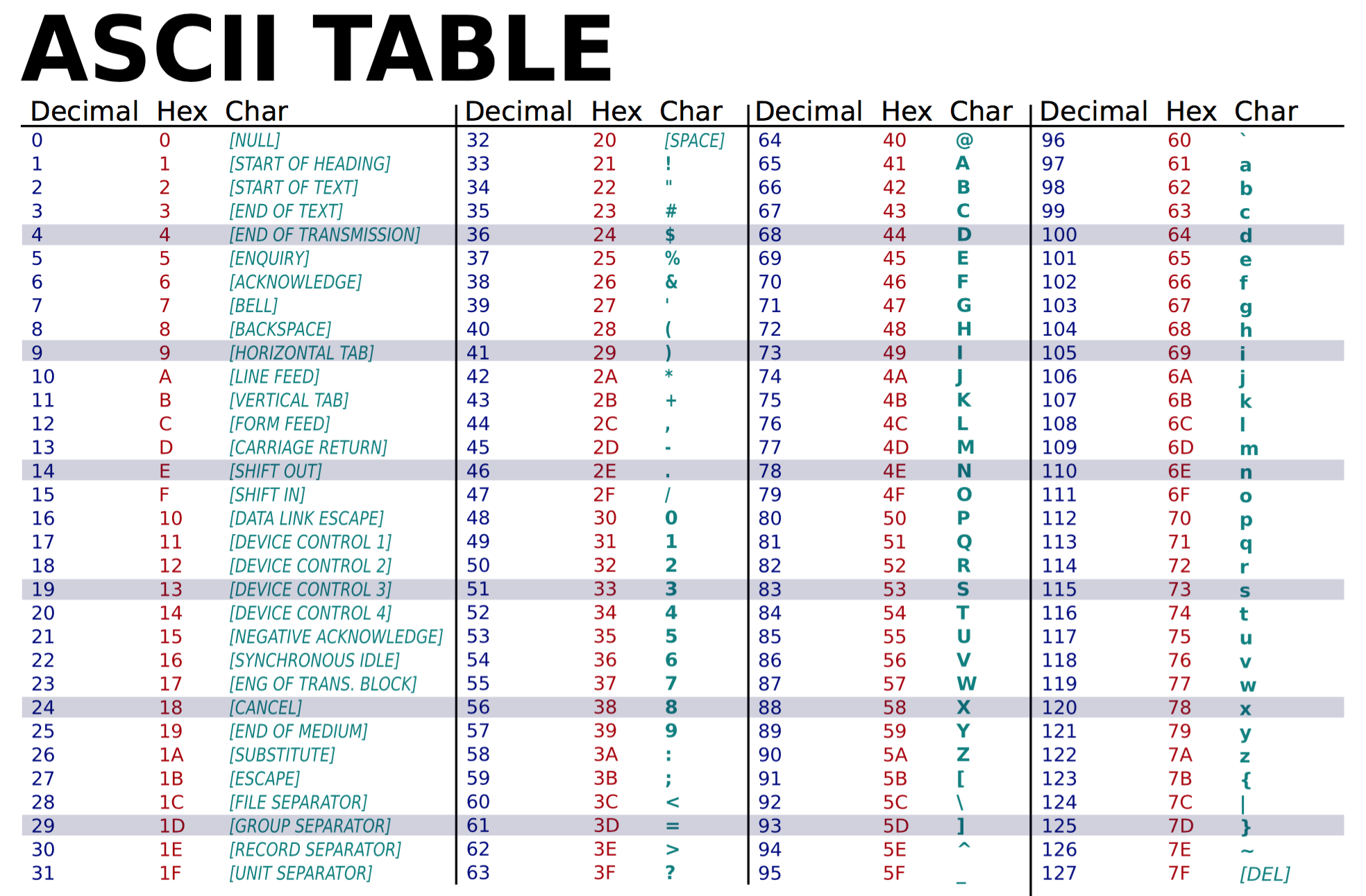
Looking at a UTF-8 or ASCII table, you can see that "A"
corresponds to 65 and "Z" to 90, while lowercase "a" corresponds
to 97 and "z" to 122. That means that Python will do the
following weird things: (Remember that # is a
comment and Python ignores anything that comes after on the same
line.)
>>> "A" < "B" # this looks good
True
>>> "a" < "b" # this looks too
True
>>> "z" < "b" # this is also fine
False
>>> "A" < "a" # hm, this doesn't seem right
True
>>> "Z" < "a" # OK this is wrong
True
>>> "A".lower() # the answer is to use lower()
'a'
>>> "A".lower() < "a".lower() # better
False
>>> "Z".lower() < "a".lower() # Great!
False
So the moral of the story is to use
lower() on
strings when you are trying to compare them for alphabetical
order.
Images and files; encoding, decoding, transcoding; glitch
This week we're going to pick up on some ideas from the reading for this week and look at some ways to experiment with those ideas with actual programs. In particular, we're going to look at some ideas from the Lev Manovich text: digital objects as numerically encoded, modularity in the form of re-usable files and chunks of code, transcoding from one file format to another, and the easy variability of digital objects. In the background will be ideas from Kittler about encoding, and ideas about glitch techniques.
In all this, we'll be working through hands-on experiments and engagement with formal qualities of the digital, to better understand the digital formalism that is the them of this unit, and to offer you opportunities for creative expression through code. With these techniques you'll be working toward opportunities not to creatively produce digital objects yourself, but rather to create code that can generate a range of creative possibilities, of which you specify the parameters.
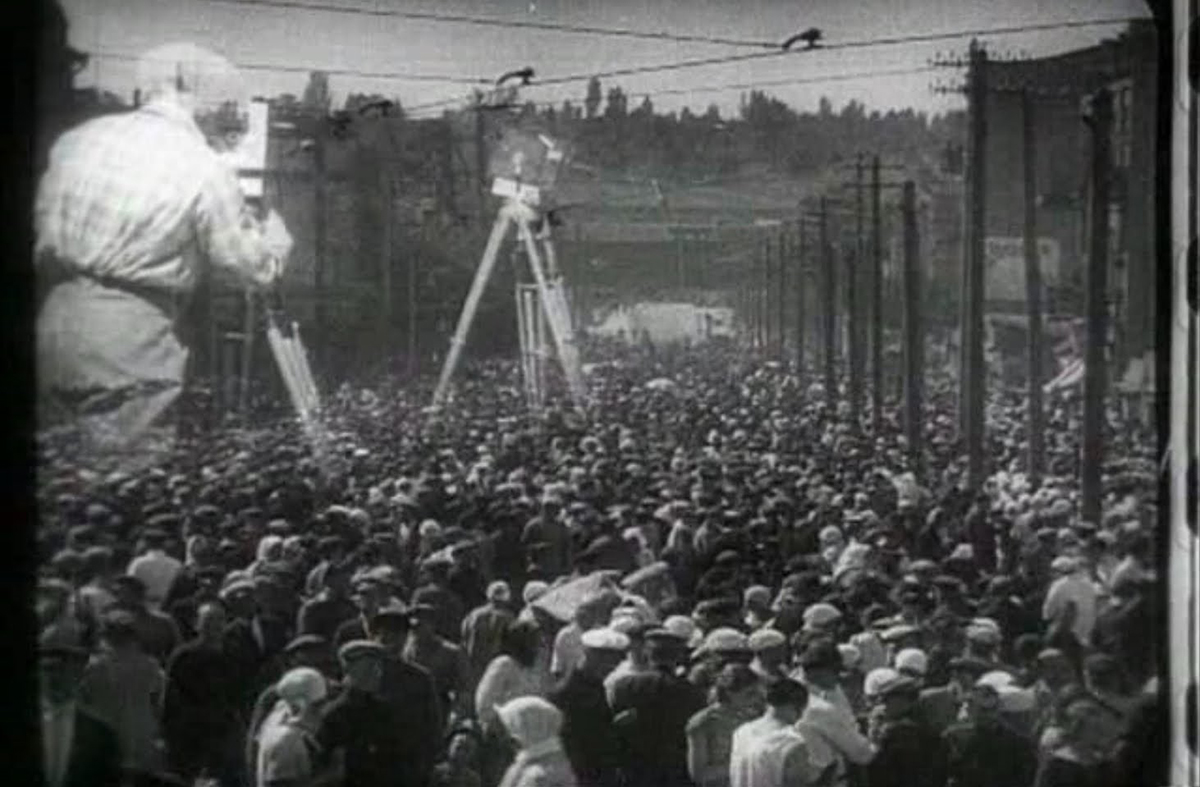 A still image from Dziga Vertov's 1929 film, "Man with a Movie
Camera." In the Prologue to The Language of New
Media, Manovich uses this film to talk about the
digital. This image shows Vertov's collage techniques —
highly innovative at the time. We'll be playing with this type
of composability in the examples below.
A still image from Dziga Vertov's 1929 film, "Man with a Movie
Camera." In the Prologue to The Language of New
Media, Manovich uses this film to talk about the
digital. This image shows Vertov's collage techniques —
highly innovative at the time. We'll be playing with this type
of composability in the examples below.
Variability on the command line
To start, let's look at how you can leverage the power of the command line interface to make your programs more dynamic, and able to respond to user input.
On the command line, we process user input
as arguments: bits of text that follow after
the command that you type. You have already seen and
used arugments on the command line. For
example, cd exercise-3. In this case,
the string exercise-2
is an argument to
the cd command. It tells
the cd command what to do — which
directory to change to. Without the argument,
the cd command would only ever be able
to do one thing. To be useful, we want to indicate to it which
directory we want to change to. That is what command
line arguments are for.
Fortunately, Python makes it very easy to work with command line
arguments. By using the sys library, which is short
for "system". This is a library that contains various utilities
for dealing with the computer and operating system within which
your code is running.
To get started, create a new file in Atom and type the following lines:
import sys

print( sys.argv )

print( len(sys.argv) )
Make a new directory (a new folder) for Exercise 3, and save
this new file into that folder. You could call
it arguments.py. Now, cd
into your new directory, and run this new program. For example:
$ python arguments.py spaghetti meatballs tomato sauce parmessanThe last five words obviously are completely made up. You can type whatever you'd like here, and you can take more or fewer words as you wish. The output that I see when I do that is:
['arguments.py', 'spaghetti', 'meatballs', 'tomato', 'sauce', 'parmessan']
6
But obviously if you typed different arguments, you'll see something different.
So far we're merely printing out the arguments, as well as a count of how many there are. Let's actually do something useful with them. (Remember, new code is in blue.)
import sys
from PIL import Image

print( sys.argv )

print( "Arguments count: " + str(len(sys.argv)) )

img = Image.open( sys.argv[1] )

print("You typed the filename: " + sys.argv[1] )
print("This is a " + img.format)
print(img.format_description)
print("Size: " + str(img.size) )
Now, if you run this and specify an image file in the same directory, you will see some useful information. For example:
$ python arguments.py fire.jpg
['arguments.py', 'fire.jpg']
Arguments count: 2
You typed the filename: fire.jpg
This is a JPEG
JPEG (ISO 10918)
Size: (720, 480)
If you type a filename that doesn't exist, you will receive an error. Or if you type a file that is not an image, you will also receive an error. And if you don't type any arguments, you will also receive an error. Lots of errors. Some of these are too complicated to prevent right now, but one error we can easily handle:
import sys
from PIL import Image

print( sys.argv )

print( len(sys.argv) )

if len(sys.argv) != 2:
    exit("This command requires one argument: the name of an image file")

img = Image.open( sys.argv[1] )

print("You typed the filename: " + sys.argv[1] )
print("This is a " + img.format)
print(img.format_description)
print("Size: " + str(img.size) )
That should make this a slightly more user-friendly command.
Transcoding
Now let's think about transcoding: translating a digital object from one encoding scheme into another. For example, converting one type of image file into a different type.
The Python Image Library (PIL, a.k.a. Pillow) makes this quite
easy. When you try to save a file using Pillow,
the save() command examines the name of the file
that you specify, tried to determine what type of encoding is
implied by that, and automatically converts the image to this
encoding before saving. Quite convenient.
Let's continue with the above example:
import sys
from PIL import Image

print( sys.argv )

print( len(sys.argv) )

if len(sys.argv) != 2:
    exit("This command requires one argument: the name of an image file")

img = Image.open( sys.argv[1] )

print("You typed the filename: " + sys.argv[1] )
print("This is a " + img.format)
print(img.format_description)
print("Size: " + str(img.size) )

img.save( sys.argv[1] + ".jpg" )
img.save( sys.argv[1] + ".gif" )
img.save( sys.argv[1] + ".tiff" )
img.save( sys.argv[1] + ".png" )
Try running that command, specify an image filename, and see
what happens. Type ls after running it
to see.
When I do this, I see additional files created in my directory:
fire.jpg.gif
fire.jpg.jpg
fire.jpg.png
fire.jpg.tiff
and I'm able to open these to view them.
The "double" extension shouldn't be an issue. Your operating system will pay attention the last few characters to determine the file type. But if that bothers you, you could add this code to better name the files:
import sys
from PIL import Image
import re

print( sys.argv )

print( len(sys.argv) )

if len(sys.argv) != 2:
    exit("This command requires one argument: the name of an image file")

img = Image.open( sys.argv[1] )

print("You typed the filename: " + sys.argv[1] )
print("This is a " + img.format)
print(img.format_description)
print("Size: " + str(img.size) )

base_filename = re.sub("\.[a-zA-Z0-9]*", "", sys.argv[1])

img.save( base_filename + ".jpg" )
img.save( base_filename + ".gif" )
img.save( base_filename + ".tiff" )
img.save( base_filename + ".png" )
(Remember that changed code will be in orange.)
Of course, this transcoding file converter tool is not actually that useful, since you could easily do the same thing in Preview (on Mac) or Microsoft Paint (on Windows). Although the potential usefulness of this idea comes into play if you needed to batch convert many files from one format to another. We'll talk next week how you can open many files at once.
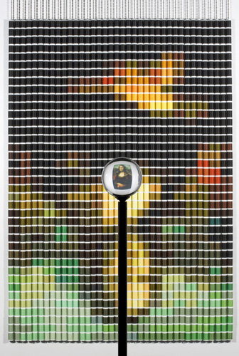 Devorah Sperber, "After the Mona Lisa
8."
Devorah Sperber, "After the Mona Lisa
8." Numerical coding: the pixel
Let's move on to think about the ways that digital objects are always represented internally to digital machinery as collections of numerical data. In particular, let's focus on digital images.
Digital images are comprised of pixels. These are essentially the atomic unit of digital imagery.
There are many different types of digital image files, called formats. You already know many of these: JPEG, PNG, TIFF, GIF, bitmaps, etc. Each of these different formats uses different techniques and algorithms for encoding a visual image as digital data. But you can think of all these digital images as comrpised of pixels, each one a small dot of color, arranged in a grid, each dot of color encoded as a numberical value. Strictly speaking, not all images are precisely represented as grids of pixels because many image formats use compression algorithms, which are efficiency tricks to allow an image to be comprised of less data, and hence a smaller file size. JPEGs are a prime example. But even for image formats that use compression, when you are working with images in computer programs, they all nearly always get translated into grids of numerical pixel values to be manipulated by computer program code.
Internal to most computer programs, you can think of the pixels of an image either arranged in a grid, with rows and columns, or, as a long list, in which all the rows of the grid are concatenated altogether into one long list.
Generally, the first pixel of an image is the dot located
visually at the top-left corner of the image. In a list, this
will be the first item, usually indicated by 0 in
most computer code. This is called the index of
the list. But when we're thinking about pixels in a grid, each
pixel will be indicated
by two indices, two numbers, refered
to as coordinates.
In most computer graphics contexts, the top-left corner of the
pixel grid is indicated with 0,0. The horizontal dimension is
always specified first and is referred to as x, and
the vertical dimension is always specified second and is
referred to as y.
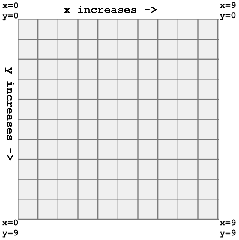
What would be the coordinates of this pixel?
It would be 2,3 — remember, we start counting
from 0,0.
What about the coordinates of this pixel?
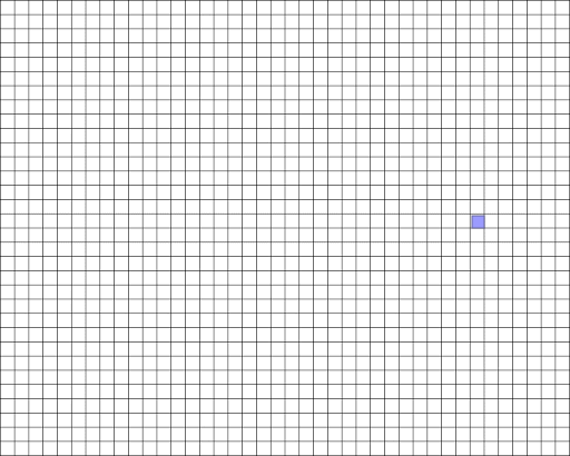
I would not recommend actually trying to count those! Instead
you can approximate. Maybe x=30
and y=15?
Computers require us to be precise, but we can comply with that precision while also being loose and approximate in achieving the goals that we're working toward. We can leave space to play, experiment, estimate, and work by trial-and-error.
The numbers of a pixel. Each pixel is usually represented by 1, 3, or 4 numbers. When one number, it corresponds to a shade of gray. When three numbers, it corresponds to red, green, and blue, which combine to form all the colors that a system can display. When four numbers, the fourth correponds to opacity, usually referred to as alpha: how see-through is this pixel.
Each pixel value generally goes from 0 to 255. Why?
As everyone knows, computers represent numerical values internally with binary numbers. Binary counting goes like this:
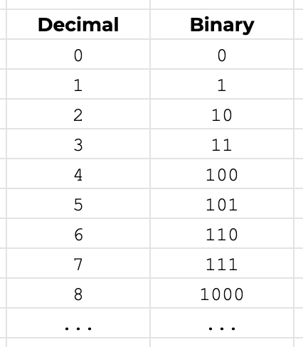
n digits in binary can
represent 2n-1 values. That means that
255 can be represented by eight binary digits. You may already
know that eight binary digits (called bits)
together are called a byte, and are a common
unit in computing. So, each pixel is represented by one, three,
or four bytes, depending on the type of color,
as described above.
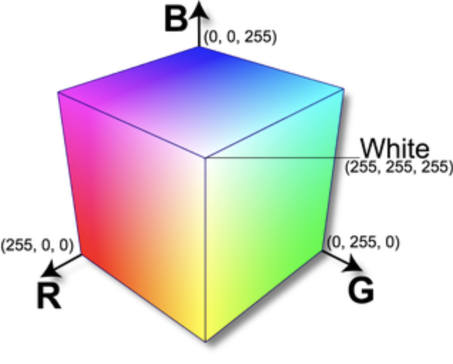
Thinking of color as space. I said that pixels are represented by three color components (red, green, and blue), and that is not always true. There are other models that we think of for representing color. Thinking about these it can be useful to imagine them spatially. In the diagrams below, on the left, we have R, G, B space, as a cube. Pay attention to how red, green, and blue are specified, and how they combine. On the right side is an alternative model called Hue, Saturation, Value. In this scheme, hue is represented by a value 0-360 corresponding to moving around the circular part of this cone; value moves up corresponding to how light or dark the color is; and saturation corresponds to the distance from the center to the edge of the circle. A color with low saturation appears more gray, brightness determines whether that gray would be more white or black, and hue is the actual shade of the color.
I share this with you because when working with color in computer programs, it is often much easier to do more powerful things using the HSV model. With this representation, we can have one number ranging from 0 to 360 to represent all colors of the spectrum: red, orange, yellow, green, blue, indigo, violet ("ROY G BIV"). With the RGB model, moving through the spectrum like this would be very difficult. We'll see some examples of this in our code for today.

Making numerical images by pattern
Let's start working with digital image objects in the most rudimentary way: by manipulating lists of pixels.
As you working with code and computers, you will start to realize that often the most "basic" way of doing something turns out to be the most complicated. The more we try to strip away layers of complexity in computing, the harder tasks become. For example, so-called "high level" programming languages (like Python or Java) are much easier to write than "low level" languages (like C or assembly). All those layers usually add ease of use. They automate the minutia and details of tasks. But working with higher level parts of the system means we often don't get to experience how computers work at more granular levels. One of the things we'll do in this first unit of the semester as we focus on digital formalism is grapple with some of these lower levels.
Let's start by creating a very small image by building up a list of pixels. Create a new file in Atom and type the following:
Example 1: Creating a simple 10x10 image
import sys
from PIL import Image

if len(sys.argv) != 2:
    exit("This program requires one argument: the name of the image file that will be created.")

# Make a new 10x10 image
img = Image.new("RGB", (10,10) )

img.save(sys.argv[1])
Try running this. First of all, you'll see that if you don't type one argument you get a helpful error message. But then you should see that whatever filename you pass will be created as a tiny digital image, that is all black. Let's add some color to it by creating pixels:
import sys
from PIL import Image

if len(sys.argv) != 2:
    exit("This program requires one argument: the name of the image file that will be created.")

# Make a new 10x10 image
img = Image.new("RGB", (10,10) )

data = []
for i in range(100):
    pixel = (i, 0, 0)
    data.append( pixel )

img.putdata(data)

img.save(sys.argv[1])
With this code, we're making a new array. Then we are looping
from 0 to 99. That's because a 10x10 image will require 100
pixels, and remember that in computer programs lists almost
always start with 0. Inside that loop, as the
variable i increases from 0 to 99, we're
using i as the red component of a pixel value in
the variable called pixel, then
using append() to add that to a list. Finally, when
the loop is complete, we use a Pillow command
called putdata() to add that list of pixels into
the new image.
Run that and see what it looks like. If you open the resulting image with a program like Preview and zoom in, you should see something like this:
Can you try to do some more interesting things with these pixels values? Here's an attempt:
import sys
from PIL import Image

if len(sys.argv) != 2:
    exit("This program requires one argument: the name of the image file that will be created.")

# Make a new 10x10 image
img = Image.new("RGB", (10,10) )

data = []
for i in range(100):
    pixel = (i, 0, 255-i)
    data.append( pixel )

img.putdata(data)

img.save(sys.argv[1])
What other patterns can you create with that loop?
As a next step, try simply making a larger image. Here I'll make a 400x400 pixel image. That means 160,000 pixels total:
import sys
from PIL import Image

if len(sys.argv) != 2:
    exit("This program requires one argument: the name of the image file that will be created.")

# Make a new 400x400 image
img = Image.new("RGB", (400,400) )

data = []
for i in range(160000):
    pixel = (i, 0, 255-i)
    data.append( pixel )

img.putdata(data)

img.save(sys.argv[1])
This works in some sense. If you open the resulting image and zoom in you'll see a thin stripe of gradient in the top row of the image. But technically this has some errors. The pixel values are going to get very large as the loop increases, larger than 255. So this might create some glitchy images, depending on the image format.
The modulo operator (%). One way
you could improve on this behavior is to use the modulo
operator: %. This symbol calculates a
remainder.
So for example: 33 % 10 calculates the remainder
when 33 is divided by 10, and the result is 3. (10 goes in to 33
three times, with a remainder of 3.)
This is a very powerful idea in computer science and computer programming. If you ever have a variable that you are incrementing, but you want to constrain it to not exceed some maximum value, you can use modulo.
Have a look at another example and step through to make sure you understand what's going on here:
>>> for i in range(10):
...   print(i % 3)
...
0
1
2
0
1
2
0
1
2
0
When i is 0, 1, or 2, the remainder
when i is divided by 3 is simply 0, 1, and 2,
respectively. (e.g. 3 goes in to 2 zero times, with a remainder
of 2.) But when i equals 3, the remainder is 0
— because 3 goes in one time, with no remainder. And
when i equals 4, 3 goes in one time with remainder
1. And the pattern continues.
We can use this in our pixel example by incrementing a looping
variable, and applying a % 255 to ensure that the
variable never increases beyond 255:
Example 2: Introducing the modulo operator
import sys
from PIL import Image

if len(sys.argv) != 2:
    exit("This program requires one argument: the name of the image file that will be created.")

# Make a new 400x400 image
img = Image.new("RGB", (400,400) )

data = []
for i in range(160000):
    pixel = (i%255, 0, 0)
    data.append( pixel )

img.putdata(data)

img.save(sys.argv[1])
If you run this, you should see a 400x400 image comprised of small gradients as the red component of the pixel values increase to 255 and then reset to 0.
Play with this new technique and see what you can get. What if you use different modulo values on the red, green, and blue components.
Pixels on the x,y grid. Remember, we can work with pixels on the x,y grid, horizontally and vertically as well. Not just one single list of pixels.
Create a new file in Atom and type the following:
Example 3: Working with pixels on as a grid
import sys
from PIL import Image

if len(sys.argv) != 2:
    exit("This program requires one argument: the name of the image file that will be created.")

# Make a new 400x400 image
img = Image.new("RGB", (400,400) )

for y in range(400):

    for x in range(400):

        pixel = (x % 255, 0, y % 255)
        img.putpixel( (x,y), pixel )

img.save(sys.argv[1])
This code, called a nested loop, first loops
from 0 to 400 incrementing y each time, and each
time it increments y, it then loops again from 0 to
400, incrementing x each time. That means the code
inside the inner loop will operate on all pixels
one at a time, based on their x,y values. Here I'm
using x to control the red value,
and y to control the blue. Run this and see what
that pattenr looks like.
x,
from left to right, and blue increases with y, from
top to bottom.
Modulo is also very useful to determine even and odd
numbers. If n % 2 is zero, that
means n is divisible by 2, which means that it is
even. Similary if n % 3 is zero, that means it is
divisible by 3, and so on. We can use this fact to create
interesting repetitions and striping behavior:
Example 4: Using modulo and the pixel grid to make stripes
import sys
from PIL import Image

if len(sys.argv) != 2:
    exit("This program requires one argument: the name of the image file that will be created.")

# Make a new 400x400 image
img = Image.new("RGB", (400,400) )

for y in range(400):

    for x in range(400):

        r = 0
        b = 0
        if x % 50 == 0:
            b = 255

        if y % 20 == 0:
            r = 255

        if y % 30 == 0:
            r = 255
            b = 255

        pixel = (r, 0, b)
        img.putpixel( (x,y), pixel )

img.save(sys.argv[1])
As a last step here, we can use the modulo
operator not just checking equality (==)
but checking ranges, with <
and >. Have a look at this example and its
output:
Example 5: Using modulo, the pixel grid, and greater than / less than operators
import sys
from PIL import Image

if len(sys.argv) != 2:
    exit("This program requires one argument: the name of the image file that will be created.")

# Make a new 400x400 image
img = Image.new("RGB", (400,400) )

for y in range(400):

    for x in range(400):

        r = 0
        g = 0
        b = 0
        if x % 50 > 25:
            r = 255

        if y % 50 > 25:
            b = 255

        if x % 100 > 50 and y % 100 > 50:
            g = 255

        pixel = (r, g, b)
        img.putpixel( (x,y), pixel )

img.save(sys.argv[1])
Combining images
This is as far as we got in class. I encourage you to play with the below examples while doing the homework for this week, and we'll pick up here next week in class.
Example 6: Combining images
import sys
from PIL import Image

if len(sys.argv) != 3:
    exit("This program requires two arguments: the name of two image files to combine.")


# open both images
img1 = Image.open( sys.argv[1] )
img2 = Image.open( sys.argv[2] )

# resize both images so they are no bigger than 400x400
# but preserve the original aspect ratio
img1.thumbnail( (400,400) )
img2.thumbnail( (400,400) )

# make a new image 600x600, with a white background
new_image = Image.new( "RGB", (600,600), "white" )

# paste in the first image to the upper-left corner (0,0)
new_image.paste(img1, (0,0) )

# paste in the second image, to (200,200)
new_image.paste(img2, (200,200) )

# save the resulting image
new_image.save("new.jpg")
Example 7: Combining images with transparency
import sys
from PIL import Image

if len(sys.argv) != 3:
    exit("This program requires two arguments: the name of two image files to combine.")


# open both images
img1 = Image.open( sys.argv[1] )
img2 = Image.open( sys.argv[2] )

# resize both images so they are no bigger than 400x400
# but preserve the original aspect ratio
img1.thumbnail( (400,400) )
img2.thumbnail( (400,400) )

# make a new image 600x600, with a white background
# Note that this image now has an "alpha" component
new_image = Image.new( "RGBA", (600,600), "white" )

# paste in the first image to the upper-left corner (0,0)
new_image.paste(img1, (0,0) )

# add some transparency (alpha) to the second image
img2.putalpha(128)

# paste in the second image, preserving its new transparency
new_image.alpha_composite(img2, (200,200) )

# save the resulting image
# Note that we must convert it to RGB with no alpha to save it as a JPEG
new_image.convert("RGB").save("new.jpg")

# Alternatively, we could have avoided converting by saving it to a
# PNG like this (since PNGs allow alpha):
# new_image.save("new.png")
Note: I fixed the below code example after class today, so even though it was throwing an error during class, it should work for you now to run and experiment with.
Example 8: Combining images with transparency based on pixel values of the source image
import sys
from PIL import Image

if len(sys.argv) != 3:
    exit("This program requires two arguments: the name of two image files to combine.")


# open both images
img1 = Image.open( sys.argv[1] )
img2 = Image.open( sys.argv[2] )

# resize both images so they are no bigger than 400x400
# but preserve the original aspect ratio
img1.thumbnail( (400,400) )
img2.thumbnail( (400,400) )

# make a new image 600x600, with a white background
# Note that this image now has an "alpha" component
new_image = Image.new( "RGBA", (600,600), "white" )

# paste in the first image to the upper-left corner (0,0)
new_image.paste(img1, (0,0) )

# convert the second image to a new image with transparency (alpha)
img2_alpha = img2.convert("RGBA")

# modify the second image, make all bluish pixels totally transparent
# (alpha 255)
(width,height) = img2_alpha.size
for x in range(width):
    for y in range(height):
        (red,green,blue,alpha) = img2_alpha.getpixel((x,y))
        if blue > red and blue > green:
            img2_alpha.putpixel( (x,y), (0,0,0,0) )


# paste in the second image, preserving its new transparency.
# Note that this time I'm placing it at 0,0 to show the transparent overlay
new_image.alpha_composite(img2_alpha, (0,0) )

# save the resulting image
# Note that we must convert it to RGB with no alpha to save it as a JPEG
new_image.convert("RGB").save("new.jpg")

# Alternatively, we could have avoided converting by saving it to a
# PNG like this (since PNGs allow alpha):
# new_image.save("new.png")