Code as a Liberal Art, Spring 2023
Unit 1, Tutorial 2, Part B — Wednesday, February 8
This lesson builds on Unit 1, Tutorial 2 from last week. We only got part way through that lesson and some of the key concepts were a bit rushed. Make sure you review that lesson up to where we got in class. These notes revist the last few items from last week's table of contents and restate them in a much clearer way. (Hopefully!)
Images and files; encoding, decoding, transcoding; glitch
Table of contents for the topics today: (Click each to jump down to the corresponding section.)
- Data structures (lists) and control structures (loops)
- Numerical representation: the pixel
- Algorithms and images: combination
I. Data structures (lists) and control structures: loops
In Unit 1, Lesson 1 we talked about implementing our first algorithm: searching through a list of numbers or text to find a value that matched some criteria. Largest, smallest, longest, etc.
To do that, we used a data structure known as a list, and a control structure known as a loop.
In Python (as in many programming
languages), lists are used to hold a sequence
of values. Lists are indicated
with square brackets [ ] and their
individual values are separated by commas. So in the data file
that I asked you to import for that homework assignment, I
created a list with the following syntax:
number_list = [ 473, 650, 745, 569, 653, 411, 71, 920 ]
(My list in that file was much longer, but this gives you the idea.)
You can access the individual values in a list by indexing the list with a number that indicates the position of that value, starting at zero. Like this:
number_list[0]
You can use that value the same way you would use any variable:
to print(), or combine with other operators and
other variables.
You can also index a list using a variable that holds one single value. This code is indentical to the above snippet:
i = 0
number_list[i]
Why would you use a variable to index a list? Because the variable value can change, which means that you can modify it in using various control structures to implement interesting algorithms.
a. while loop
Here is how I could print each item in a list using
a control structure called a while
loop:
i = 0
while i < len(number_list):
    print( number_list[i] )
    i = i + 1
len() is a Python command that tells me the length
of a list.
Stepping through this code, I first create a variable
called i and set it to 0. Then I enter
a while loop. This will repeat all the code "in"
the loop block as long as the logic condition
in the while statement
is True. In this case, my condition is
that i is less than the length
of number_list. If it is, I print the item in the
list that is indexed by the value
of i. First that is the 0 item (the
first), then I increment i
by 1, so now i equals 1,
and the loops repeats, going back to the
condition. i is still less than the length of the
list, so the code in the while statement runs, and
I print the item in the list indexed by the value
of i, which is 1, i.e. the second item
in the list. This repats for i equal
to 2, 3, etc, until
finally i is longer than the length of the list,
the conditional in my while statement
return False, and the loop stops repeating.
b. for loop
This pattern, using a loop to iterate through
each item in a list, is such a common pattern in
coding, that Python (and most programming languages) have
a control structure to make a shortcut for
this: the for loop. Here is how to implement the
above algorithm with this new control structure:
for n in number_list:
    print( n )
These are identical and you can use whichever is clearer and
easier for you to use. I find that studnets often like working
with while loops at first, since the syntax
makes it a little clearer what is going on. But quickly people
start preferring for loops because they are more
concise.
while loops are also more error prone. If you
forget that increment line (i = i +
1), which is a very common mistake, then you will get
an infinite loop, which repeats and never
ends. for loops help prevent this error
possibility.
More on data structures later
We will talk more about data structures in Unit 2. For now, let's use this knowledge to move on and develop some techniques to work with images.
(jump back up to table of contents)I. Numerical representation: the pixel
Let's move on to think about the ways that digital objects are always represented internally to digital machinery as collections of numerical data. In particular, let's focus on digital images.
As we talked about last week, digital images are comprised of pixels. These are essentially the atomic unit of digital imagery. You can think of a pixel as a small dot of color, encoded as a numberical value, arranged in a grid.
Even though digital images are generally view as a grid, in 2D, i.e. with width and height, internal to most computer programs, the data of a digital image is stored in one continuous chunk of data. This means that in our code, we have the option of working with digital image data either as a grid with width and height, or as one long chunk of data, which we can operate on as a list.
First, we'll build on our current control structure and data structure knowledge to experiment with pixels as stored in a list. But before that, we have to pause and think about numerical representation and how pixels store color values.
a. Color modes
The numbers of a pixel. Each pixel is usually represented by 1, 3, or 4 numbers. When one number, it corresponds to a shade of gray. When three numbers, it usually corresponds to red, green, and blue, which combine to form all the colors that a system can display. When four numbers, the fourth correponds to opacity, usually referred to as alpha: how see-through is this pixel.
Each pixel value generally goes from 0 to 255. (See last week's class notes for an explanation of why 255.)
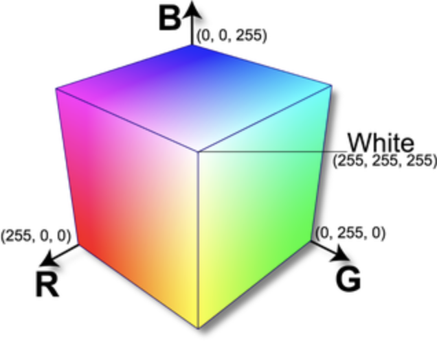
Thinking of color as space. When working with color as RGB (red, green, and blue components), it is sometimes helpful to think of color as arranged in 3D space, with red, green, and blue values along the three axes. Some digital tools (like Adobe Creative Suite) offer you similar views. This can help you think about how to specify color values. You can also use tools like Google's Color Picker to help you select RGB color values.
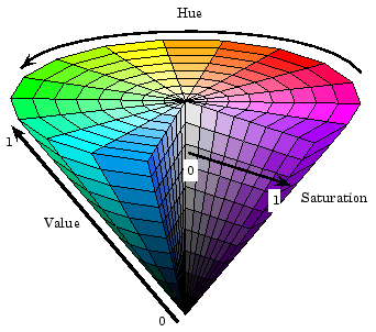
On the right, the cone shape is corresponds to another common color mode: hue, saturation, and brightness (HSB). Sometimes this is referred to as HSB, which stands for hue, staturation and value.
In this mode, hue corresponds to the shade, like a rainbow or the mneumonic ROY G BIV: red, orange, yellow, blue, indigo, violet. Typically hue is represented in degrees from 0 to 360, like moving around a circle (red is represented by 0). Brightness corresponds to how much black is in the color: 0 is all black (bottom of the cone), and 100 is no black (at the top of the cone). And saturation is how much white is in the color: 0 is all white (middle of the cone) and 100 is no white (edges around the circular part of the cone). The cone can help you visualize this.
I'll show you below how you can specify color mode when working with images in Python.
When working with code and algorithms, I find HSV to be much more useful because using math and control structures like loops, I can easily move through different hues in a more natural way. Trying to move smoothly through a ROY G BIV rainbow using RGB can be very difficult. You can use whichever you'd prefer, and in different coding contexts, you might prefer one mode over another.
b. Pixels as a list: filtering
OK, now we're ready to work with numerical image data as a list of pixels color values.
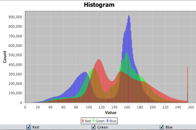

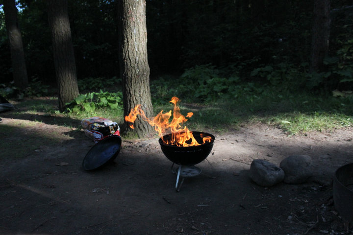
The image on the left is a histogram that shows the relative amounts of various color components (red, green, and blue) in a digital image. The image on the right is the result of a filter applied to replace all colors in the image with only 4 or 5 colors, determined based on the brightness of pixels in the original.
The code sample below opens an image and applies a filtering
algorithm which loops over the image, pixel by pixel, checking
each one for brightness. Create a new file in VS Code, let's
call it pixel_filtering.py, and type
the following:
Example 0: Filtering image pixels
from PIL import Image

img = Image.open("fire.jpg")

new_img = img.convert(mode="HSV")
new_img_data = []

for pixel in new_img.getdata():
    if pixel[2] < 50:
        new_img_data.append( (0,0,255) )
    else:
        new_img_data.append( pixel )

new_img.putdata(new_img_data)
new_img.convert(mode="RGB").save("new.jpg")
The variable img holds the image that I've
opened. Then I call .convert() on that image and
return the resulting value to a new
variable, new_img, which now holds a new image that
has been converted to the HSV color
mode. new_img_data is a new list that will hold
pixel color data for the filtered image. .getdata()
returns all the pixel color data for an image as a list, which I
can loop over with the for command. In this
loop, pixel will hold each pixel value in
turn. Note that pixel is not a keyword. It's a
veriable name that I made up and could be anything; I used this
name for clarity. Now, pixel will hold each pixel
value, and I can reference the specific componets HSV as if they
too were a list. So pixel[0] is
hue, pixel[1] is saturation,
and pixel[2] is brightness.
"Inside" my for loop, I have an if
statement that asks if pixel[2] (brightness) is
less than 50. If it is (if this pixel is dark) I set its value
to be HSV 0,0,255, which is white. Otherwise (else)
I set the pixel value in new_img_data to simply
be pixel, the unmodified original pixel value. Then
I call .putdata() to set my new list of pixel color
data into new_img, and call .convert()
to convert it back to RGB mode, then .save() to
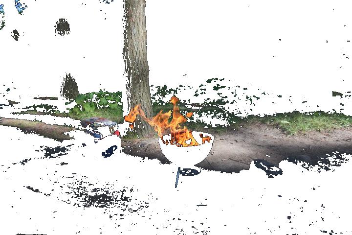
save the file. A sample output of what this looks like is below.
b. Pixels as a list: generating
Now let's explore working with algorithms to generate digital images by making numerical patterns. We can do this in the most rudimentary way possible: by manipulating lists of pixels.
Let's start by creating a very small image by building up a list
of pixels. Create a new file in VS Code, let's call
it pixel_generation.py and type the
following:
Example 1: Creating a simple 10x10 image
import sys
from PIL import Image

if len(sys.argv) != 2:
    exit("This program requires one argument: the name of the image file that will be created.")

# Make a new 10x10 image
img = Image.new("RGB", (10,10) )

img.save(sys.argv[1])
Try running this. First of all, you'll see that if you don't type one argument you get a helpful error message. But then you should see that whatever filename you pass will be created as a tiny digital image, that is all black. Let's add some color to it by creating pixels:
import sys
from PIL import Image

if len(sys.argv) != 2:
    exit("This program requires one argument: the name of the image file that will be created.")

# Make a new 10x10 image
img = Image.new("RGB", (10,10) )

data = []
for i in range(100):
    pixel = (i, 0, 0)
    data.append( pixel )

img.putdata(data)

img.save(sys.argv[1])
With this code, we're making a new array. Then we are looping
from 0 to 99. That's because a 10x10 image will require 100
pixels, and remember that in computer programs lists almost
always start with 0. Inside that loop, as the
variable i increases from 0 to 99, we're
using i as the red component of a pixel value in
the variable called pixel, then
using append() to add that to a list. Finally, when
the loop is complete, we use a Pillow command
called putdata() to add that list of pixels into
the new image.
Run that and see what it looks like. If you open the resulting image with a program like Preview and zoom in, you should see something like this:
Can you try to do some more interesting things with these pixels values? Here's an attempt:
import sys
from PIL import Image

if len(sys.argv) != 2:
    exit("This program requires one argument: the name of the image file that will be created.")

# Make a new 10x10 image
img = Image.new("RGB", (10,10) )

data = []
for i in range(100):
    pixel = (i, 0, 255-i)
    data.append( pixel )

img.putdata(data)

img.save(sys.argv[1])
What other patterns can you create with that loop?
As a next step, try simply making a larger image. Here I'll make a 400x400 pixel image. That means 160,000 pixels total:
import sys
from PIL import Image

if len(sys.argv) != 2:
    exit("This program requires one argument: the name of the image file that will be created.")

# Make a new 400x400 image
img = Image.new("RGB", (400,400) )

data = []
for i in range(160000):
    pixel = (i, 0, 255-i)
    data.append( pixel )

img.putdata(data)

img.save(sys.argv[1])
This works in some sense. If you open the resulting image and zoom in you'll see a thin stripe of gradient in the top row of the image. But technically this has some errors. The pixel values are going to get very large as the loop increases, larger than 255. So this might create some glitchy images, depending on the image format.
c. Pixels and the modulo operator %
One way you could do some more interesting stuff here is with
our old friend the modulo
operator: %.
As I've mentioned, modulo is a very powerful idea in computer science and computer programming. If you ever have a variable that you are incrementing, but you want to constrain it to not exceed some maximum value, you can use modulo. In this case, we have a variable that is looping over every pixel in the image, but we want our pixels to stay in the 0-255 range.
Have a look at another example and step through to make sure you understand what's going on here:
>>> for i in range(10):
...   print(i % 3)
...
0
1
2
0
1
2
0
1
2
0
When i is 0, 1, or 2, the remainder
when i is divided by 3 is simply 0, 1, and 2,
respectively. (e.g. 3 goes in to 2 zero times, with a remainder
of 2.) But when i equals 3, the remainder is 0
— because 3 goes in one time, with no remainder. And
when i equals 4, 3 goes in one time with remainder
1. And the pattern continues.
We can use this in our pixel example by incrementing a looping
variable, and applying a % 255 to ensure that the
variable never increases beyond 255:
Example 2: Introducing the modulo operator
import sys
from PIL import Image

if len(sys.argv) != 2:
    exit("This program requires one argument: the name of the image file that will be created.")

# Make a new 400x400 image
img = Image.new("RGB", (400,400) )

data = []
for i in range(160000):
    pixel = (i%255, 0, 0)
    data.append( pixel )

img.putdata(data)

img.save(sys.argv[1])
If you run this, you should see a 400x400 image comprised of small gradients as the red component of the pixel values increase to 255 and then reset to 0.
Play with this new technique and see what you can get. What if you use different modulo values on the red, green, and blue components.
d. Pixels as a grid
Remember, we can also work with pixels on the x,y grid, horizontally and vertically as well. Not just one single list of pixels.
Generally, the first pixel of an image is the dot located
visually at the top-left corner of the image. In a list, this
means that the index of the first pixel in the
list will be 0. But when we're thinking about
pixels in a grid, each pixel will be indicated
by two indices, two numbers, refered
to as coordinates.
In most computer graphics contexts, the top-left corner of the
pixel grid is indicated with 0,0. The horizontal dimension is
always specified first and is referred to as x, and
the vertical dimension is always specified second and is
referred to as y.

What would be the coordinates of this pixel?
It would be 2,3 — remember, we start counting
from 0,0.
What about the coordinates of this pixel?
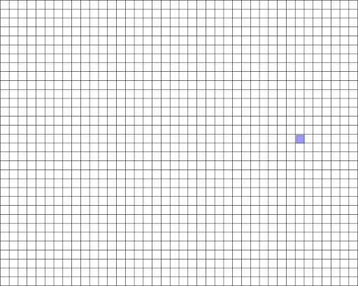
I would not recommend actually trying to count those! Instead
you can approximate. Maybe x=30
and y=15?
Computers require us to be precise, but we can comply with that precision while also being loose and approximate in achieving the goals that we're working toward. We can leave space to play, experiment, estimate, and work by trial-and-error.
Create a new file in VS Code, let's call
it pixels_grid.py, and type the
following:
Example 3: Working with pixels on as a grid
import sys
from PIL import Image

if len(sys.argv) != 2:
    exit("This program requires one argument: the name of the image file that will be created.")

# Make a new 400x400 image
img = Image.new("RGB", (400,400) )

for y in range(400):

    for x in range(400):

        pixel = (x % 255, 0, y % 255)
        img.putpixel( (x,y), pixel )

img.save(sys.argv[1])
This code, called a nested loop, first loops
from 0 to 400 incrementing y each time, and each
time it increments y, it then loops again from 0 to
400, incrementing x each time. That means the code
inside the inner loop will operate on all pixels
one at a time, based on their x,y values. Here I'm
using x to control the red value,
and y to control the blue. Run this and see what
that pattenr looks like.
x,
from left to right, and blue increases with y, from
top to bottom.
Modulo is also very useful to determine even and odd
numbers. If n % 2 is zero, that
means n is divisible by 2, which means that it is
even. Similary if n % 3 is zero, that means it is
divisible by 3, and so on. We can use this fact to create
interesting repetitions and striping behavior:
Example 4: Using modulo and the pixel grid to make stripes
import sys
from PIL import Image

if len(sys.argv) != 2:
    exit("This program requires one argument: the name of the image file that will be created.")

# Make a new 400x400 image
img = Image.new("RGB", (400,400) )

for y in range(400):

    for x in range(400):

        r = 0
        b = 0
        if x % 50 == 0:
            b = 255

        if y % 20 == 0:
            r = 255

        if y % 30 == 0:
            r = 255
            b = 255

        pixel = (r, 0, b)
        img.putpixel( (x,y), pixel )

img.save(sys.argv[1])
As a last step here, we can use the modulo
operator not just checking equality (==)
but checking ranges, with <
and >. Have a look at this example and its
output:
Example 5: Using modulo, the pixel grid, and greater than / less than operators
import sys
from PIL import Image

if len(sys.argv) != 2:
    exit("This program requires one argument: the name of the image file that will be created.")

# Make a new 400x400 image
img = Image.new("RGB", (400,400) )

for y in range(400):

    for x in range(400):

        r = 0
        g = 0
        b = 0
        if x % 50 > 25:
            r = 255

        if y % 50 > 25:
            b = 255

        if x % 100 > 50 and y % 100 > 50:
            g = 255

        pixel = (r, g, b)
        img.putpixel( (x,y), pixel )

img.save(sys.argv[1])
III. Algorithms and Images: Combination
This is as far as we got in class. I encourage you to play with the below examples while doing the homework for this week, and we'll pick up here next week in class.
Example 6: Combining images
import sys
from PIL import Image

if len(sys.argv) != 3:
    exit("This program requires two arguments: the name of two image files to combine.")


# open both images
img1 = Image.open( sys.argv[1] )
img2 = Image.open( sys.argv[2] )

# resize both images so they are no bigger than 400x400
# but preserve the original aspect ratio
img1.thumbnail( (400,400) )
img2.thumbnail( (400,400) )

# make a new image 600x600, with a white background
new_image = Image.new( "RGB", (600,600), "white" )

# paste in the first image to the upper-left corner (0,0)
new_image.paste(img1, (0,0) )

# paste in the second image, to (200,200)
new_image.paste(img2, (200,200) )

# save the resulting image
new_image.save("new.jpg")
Example 7: Combining images with transparency
import sys
from PIL import Image

if len(sys.argv) != 3:
    exit("This program requires two arguments: the name of two image files to combine.")


# open both images
img1 = Image.open( sys.argv[1] )
img2 = Image.open( sys.argv[2] )

# resize both images so they are no bigger than 400x400
# but preserve the original aspect ratio
img1.thumbnail( (400,400) )
img2.thumbnail( (400,400) )

# make a new image 600x600, with a white background
# Note that this image now has an "alpha" component
new_image = Image.new( "RGBA", (600,600), "white" )

# paste in the first image to the upper-left corner (0,0)
new_image.paste(img1, (0,0) )

# add some transparency (alpha) to the second image
img2.putalpha(128)

# paste in the second image, preserving its new transparency
new_image.alpha_composite(img2, (200,200) )

# save the resulting image
# Note that we must convert it to RGB with no alpha to save it as a JPEG
new_image.convert("RGB").save("new.jpg")

# Alternatively, we could have avoided converting by saving it to a
# PNG like this (since PNGs allow alpha):
# new_image.save("new.png")
Example 8: Combining images with transparency based on pixel values of the source image
import sys
from PIL import Image

if len(sys.argv) != 3:
    exit("This program requires two arguments: the name of two image files to combine.")


# open both images
img1 = Image.open( sys.argv[1] )
img2 = Image.open( sys.argv[2] )

# resize both images so they are no bigger than 400x400
# but preserve the original aspect ratio
img1.thumbnail( (400,400) )
img2.thumbnail( (400,400) )

# make a new image 600x600, with a white background
# Note that this image now has an "alpha" component
new_image = Image.new( "RGBA", (600,600), "white" )

# paste in the first image to the upper-left corner (0,0)
new_image.paste(img1, (0,0) )

# convert the second image to a new image with transparency (alpha)
img2_alpha = img2.convert("RGBA")

# modify the second image, make all bluish pixels totally transparent
# (meaning that alpha the fourth argument will be 0)
(width,height) = img2_alpha.size
for x in range(width):
    for y in range(height):
        (red,green,blue,alpha) = img2_alpha.getpixel((x,y))
        if blue > red and blue > green:
            img2_alpha.putpixel( (x,y), (0,0,0,0) )


# paste in the second image, preserving its new transparency.
# Note that this time I'm placing it at 0,0 to show the transparent overlay
new_image.alpha_composite(img2_alpha, (0,0) )

# save the resulting image
# Note that we must convert it to RGB with no alpha to save it as a JPEG
new_image.convert("RGB").save("new.jpg")

# Alternatively, we could have avoided converting by saving it to a
# PNG like this (since PNGs allow alpha):
# new_image.save("new.png")